Vector Databases Deep Dive


Recall that the emerging LLM tech stack consists of four main layers: Data, Model, Orchestration, and Operational. This stack uses in-context learning to tailor pre-trained Large Language Models (LLMs), such as OpenAI's GPT-4 and Meta's Llama 3, for your specific applications. As part of the Data layer, vector databases play a crucial role in Retrieval-Augmented Generation (RAG), allowing you to enhance an LLM's knowledge with contextual or proprietary data.
In this article, we’ll get a deeper understanding of vector databases:
An embedding is a numerical representation that captures semantic meaning and is expressed as a vector. Embeddings can be compared to see how related they are. Embeddings of unstructured data can be quickly classified and searched with specialized techniques.
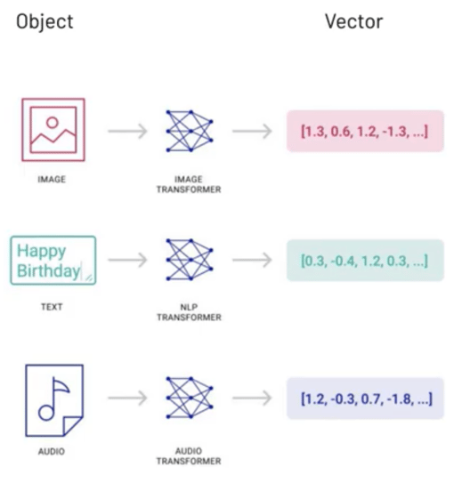
A diagram showing vector data. Source: Pinecone The Rise of Vector Data
A transformer is typically used to create the embeddings. For example, OpenAI offers embedding models for turning text, such as natural language or code, into embeddings. However, if the input data is huge in size, then chunking is needed to break up the input data into smaller fragments. At the time of writing, OpenAI's text embedding models have a maximum input size of 8,192 tokens.
Vector databases use a combination of different algorithms to enable the approximate nearest neighbor (ANN) approach. A common pipeline involves the following stages: indexing, querying, and filtering.
Vector databases focus on storing and retrieving high-dimensional embeddings, alongside the original content chunks. Unlike relational databases that create indexes based on the table columns, vector databases utilize specialized algorithms for indexing.
The indexing algorithms help improve vector search in two main ways:
Read on to learn more about each indexing algorithm.
Stores vectors in their original form.
Separates the vector space into clusters, where each cluster is represented by a centroid (geometric center or arithmetic mean position). During indexing, vectors are assigned to the nearest centroid, creating an inverted index that maps centroids to lists of vectors. When searching, the query vector is first matched to the closest centroid, narrowing the search to vectors within that cluster. More clusters can improve accuracy but require additional memory and computation to maintain the index.
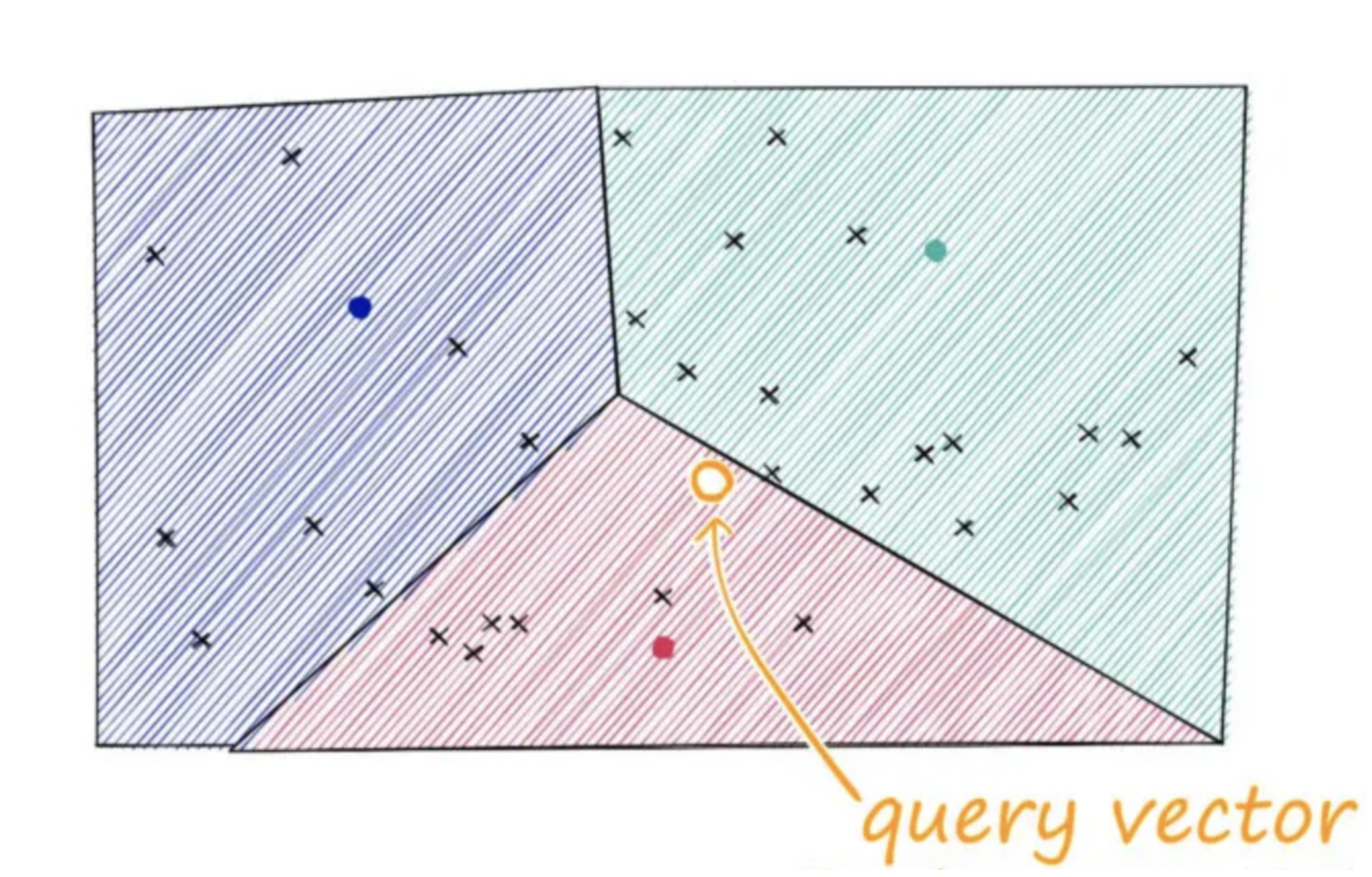
An illustration of Inverted File indexing: Source
Maps similar vectors into the same hash tables using a set of hash functions. When searching, the query vector is hashed via the same functions and compared to vectors in the same table. By reducing the search space to vectors in the same hash table, searches are quicker. The search is non-exhaustive and provides approximate results. More hash functions improve accuracy but increase search computation.
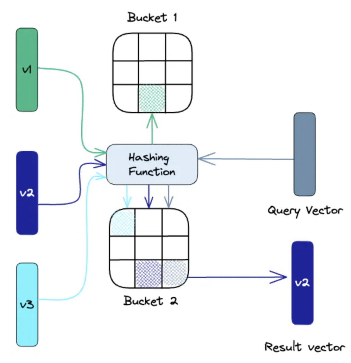
An illustration of Locality-Sensitive Hashing indexing: Source
Builds multiple binary trees by recursively splitting the vector space with random hyperplanes. During indexing, vectors are assigned to nodes based on their position relative to these hyperplanes, continuing until leaf nodes contain only a few vectors. When searching, multiple trees are traversed in parallel, using a priority queue to explore likely branches. The candidate vectors are then ranked by their true distance to the query vector. More trees improve accuracy but increase memory and build time.
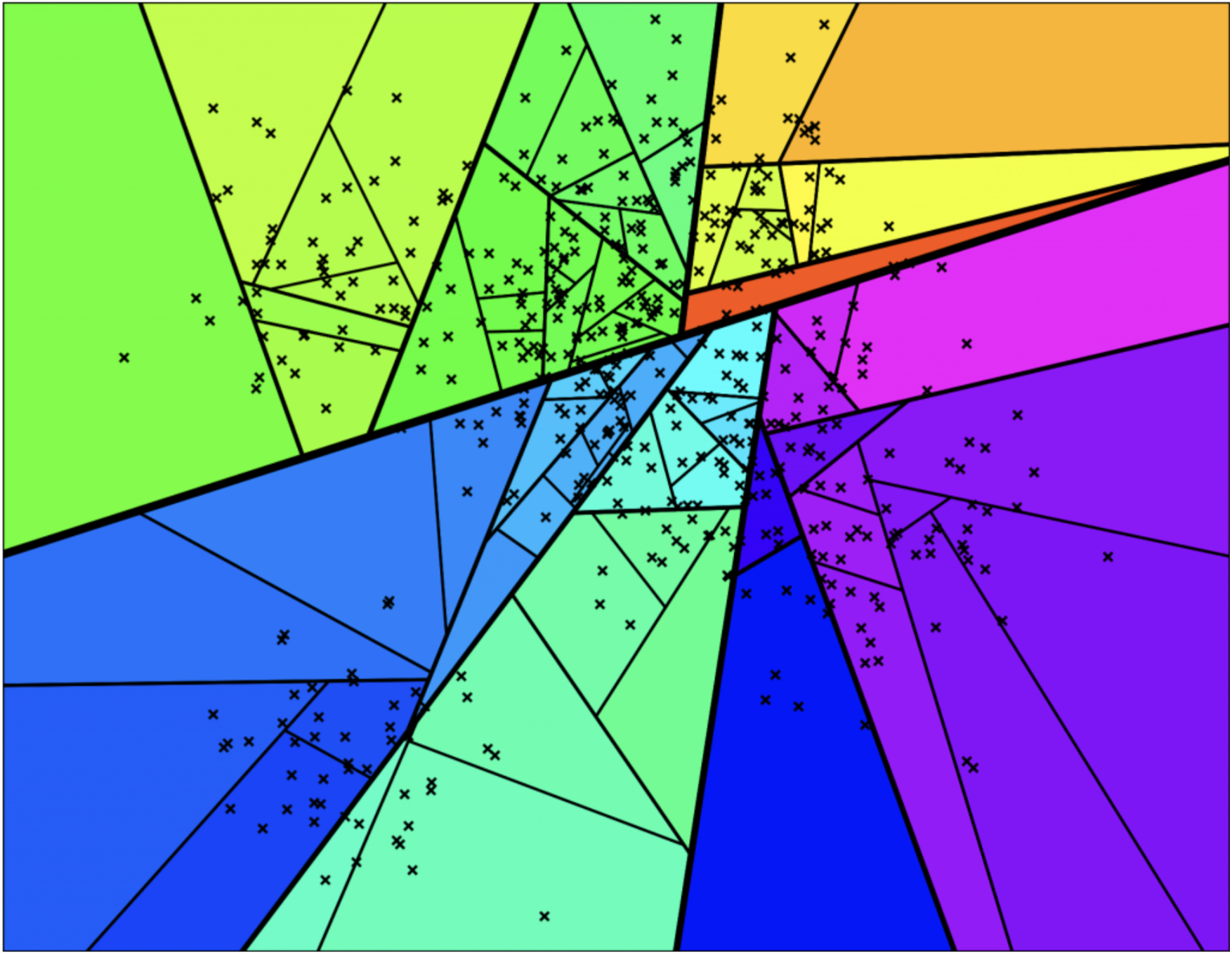
An illustration of hyperplanes used in Approximate Nearest Neighbors Oh Yeah indexing: Source
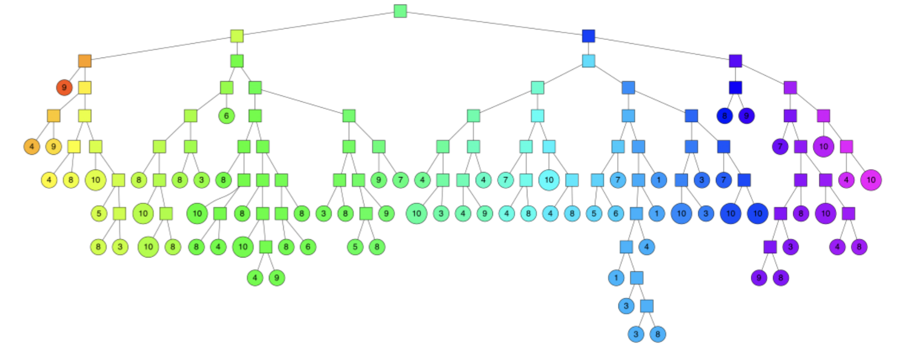
An illustration of binary trees used in Approximate Nearest Neighbors Oh Yeah indexing: Source
Creates a hierarchical, multi-layered graph structure of nodes representing vectors. Similar nodes are connected, with the top layers containing long-range connections and the bottom layers containing localized connections. During a search, the algorithm navigates down the hierarchy to find vectors most similar to the query vector. The hierarchical nature allows for efficient navigation through the search space. More connections between nodes improve accuracy but at the cost of increased memory usage and computation.
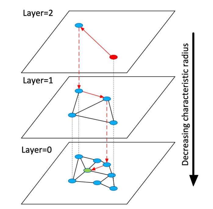
An illustration of a layered Hierarchical Navigable Small World indexing: Source
Projects high-dimensional vectors to lower-dimensional vectors using a matrix of random numbers. Calculating the dot product of the input vectors and matrix results in a projected matrix containing lower-dimensional vectors while keeping their similarity. When searching, the query vector is also simplified with the same random matrix. By reducing the data complexity while maintaining a good approximation of their relationships, searches are significantly faster. Generating a more random matrix improves the projection quality.
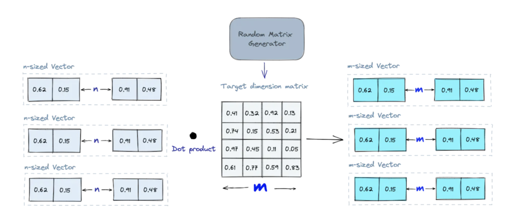
An illustration of Random Projection indexing: Source
Splits high-dimensional vectors into smaller parts, represents each part with a code, and then reassembles the parts. The code representations are generated by performing k-means clustering and collectively form a codebook. When searching, the query vector is simplified via the same process and matched against the same codebook. More codes in the codebook improve accuracy but increase search computation.
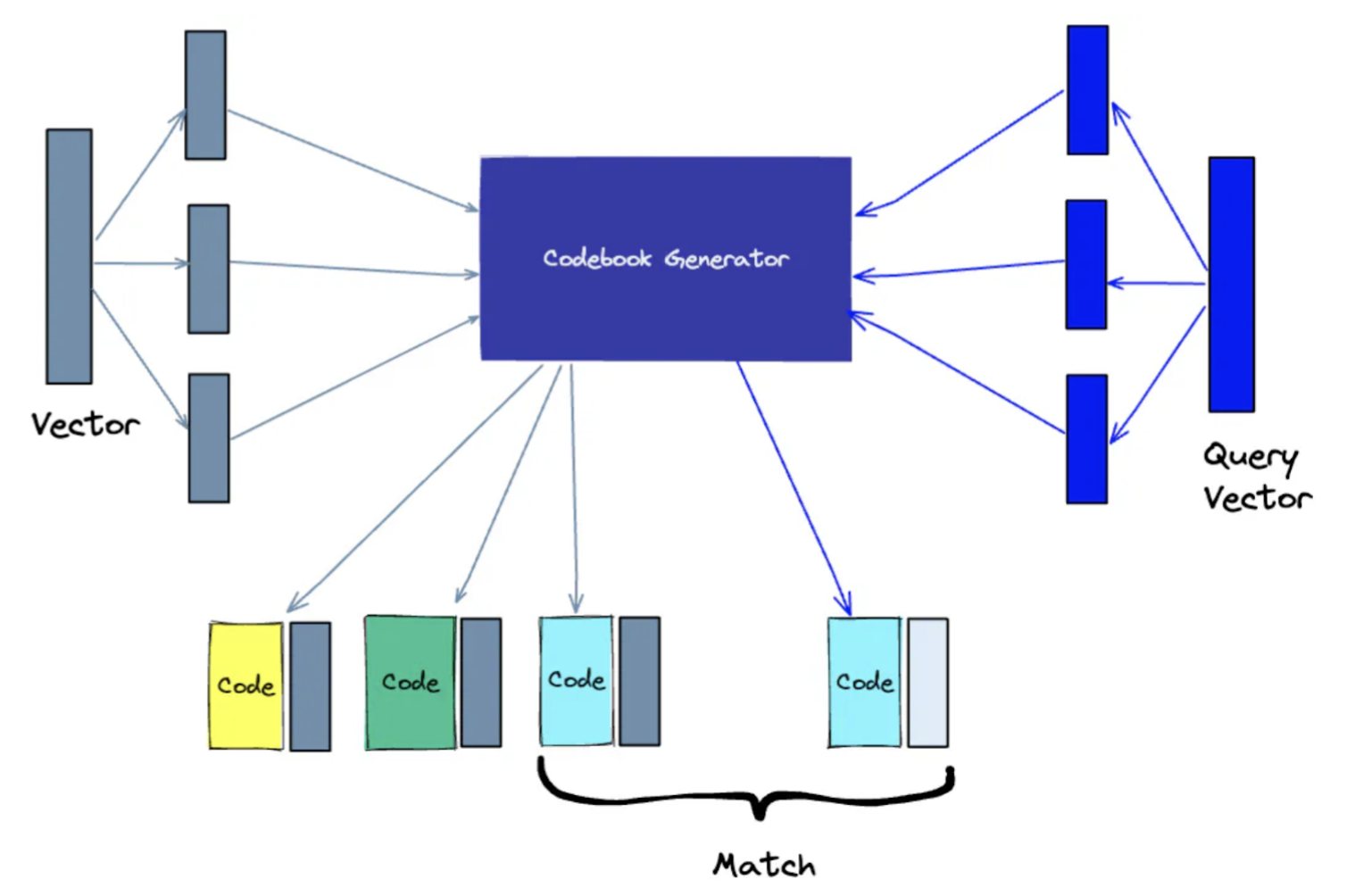
An illustration of Product Quantization indexing: Source
Compresses vectors by converting each component from a higher-precision format (e.g. 32-bit float) to a lower-precision format (e.g. 8-bit integer). This process maps continuous values to a finite set of discrete values. During indexing and search, all vectors undergo the same quantization, which reduces memory usage while approximately preserving vector relationships. Using more bits per component improves precision but increases memory requirements.
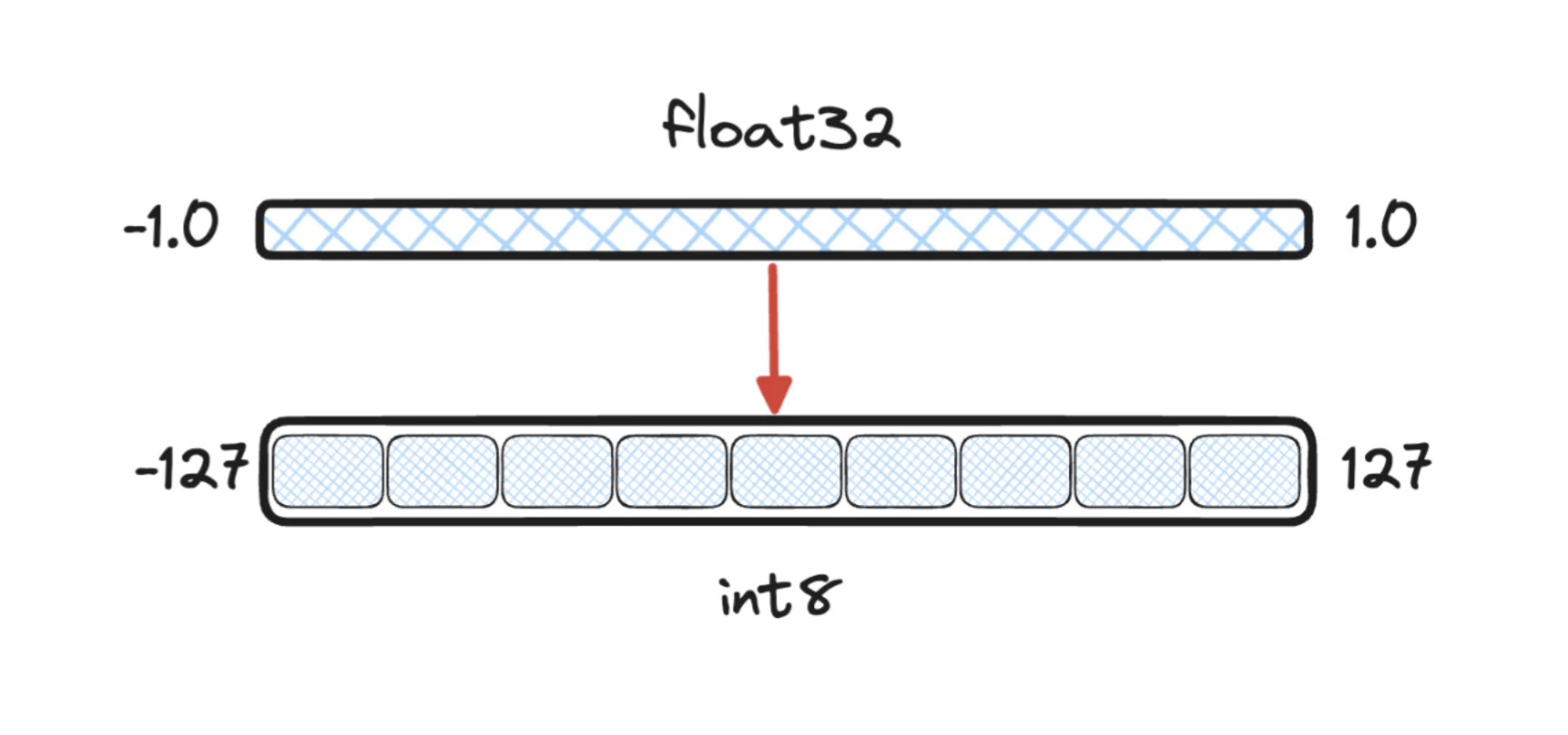
An illustration of Scalar Quantization mapping: Source
Providers of vector databases and add-ons offer different indexing options. As this is an evolving space, check out the providers' latest documentation on current indexing options available.
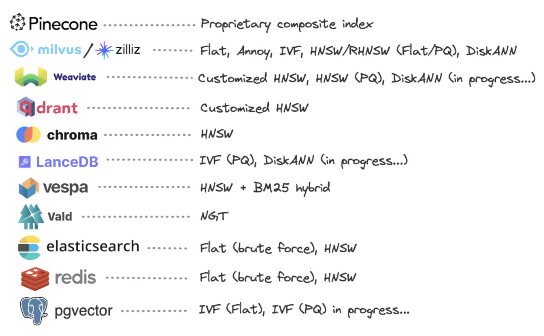
A list of available indexing options for some popular providers (non-exhaustive, as of 11/29/2023): Source
Selecting the suitable vector index depends on your specific application requirements. You need to consider various factors, such as dataset size, search quality, search speed, and memory usage. For the highest accuracy, use a Flat index, because there is no approximation error introduced from vector reduction. However, as the dataset size increases, using a Flat index means query time becomes longer. HNSW index offers good search quality and quick speed but at the cost of high memory usage. IVF index seems to be a good scalable option that offers high search quality with acceptable speed and memory usage. Some providers also offer composite indexing options that are helpful for very large datasets, such as IVF_PQ for memory-constrained applications and HNSW_SQ for high-recall applications.
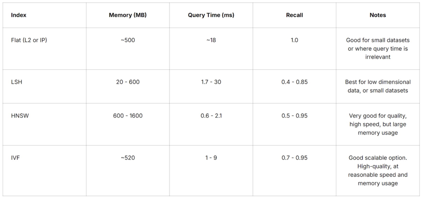
A table of vector search metrics (memory, query time, recall) for various indexes from Pinecone: Source
In addition to storing the embeddings, metadata associated with each embedding can be stored. Examples of metadata are content type, category, source, etc. Hence, vector databases typically maintain a vector index and a metadata index. Traditional indexing methods are used for indexing the structured metadata. Some common indexing methods include:
Unlike traditional databases (SQL and NoSQL) which look for exact matches, vector databases look for similar matches. The following are some common measures of similarity for comparing two vectors:
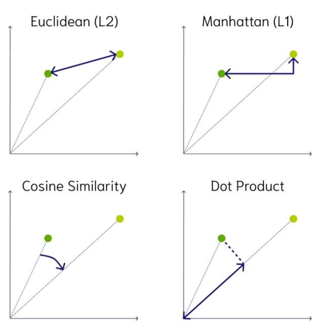
2D illustrations of vector similarity measures: Source
Aside from searching for similar vectors, vector databases can also filter the results based on a metadata query. The metadata filtering can be done before or after the vector similarity search.
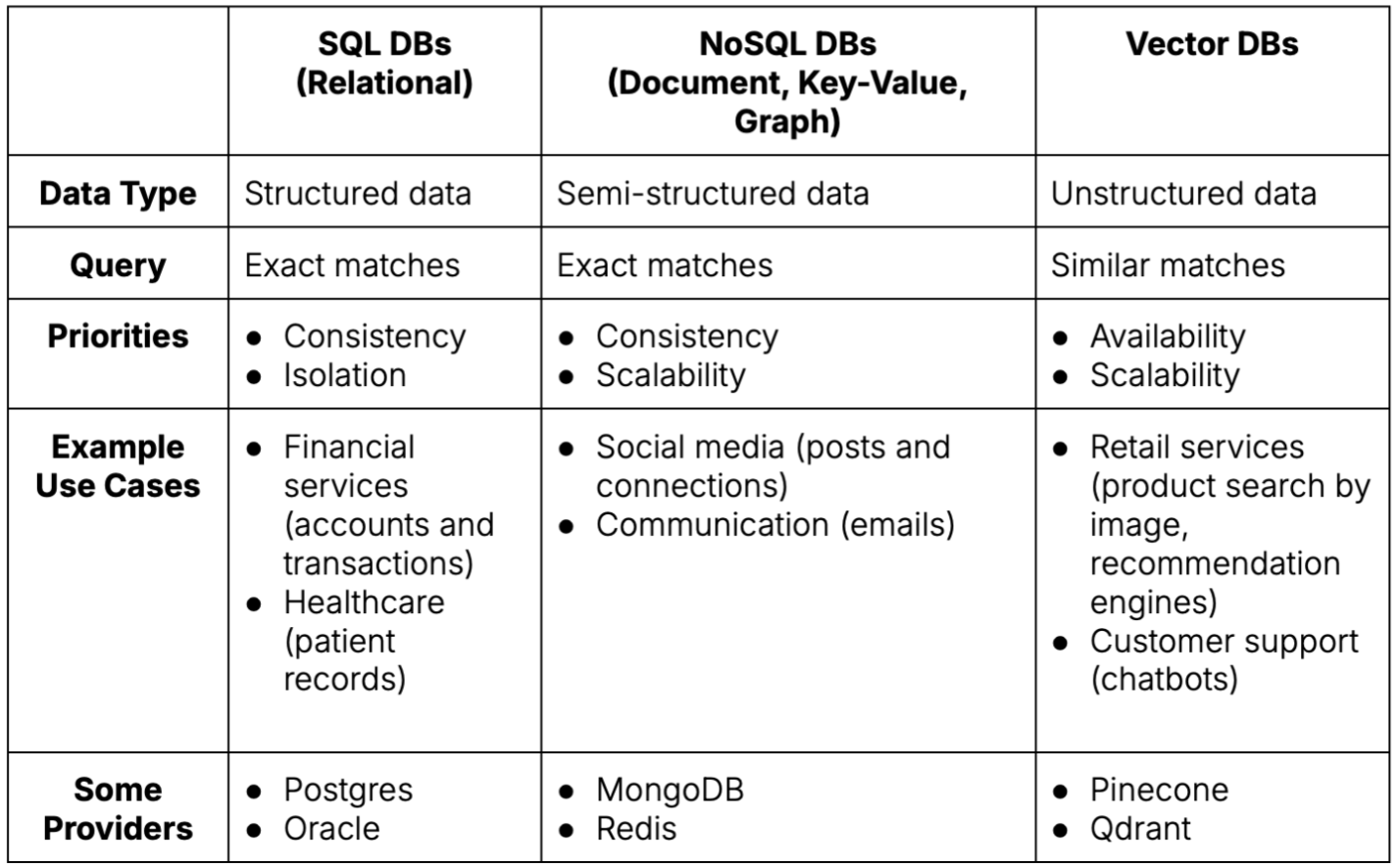
A table comparing database types across several dimensions. Source: Author
Deciding which type of database to use depends on the type of data to store and retrieve:
Different types of databases have distinct priorities:
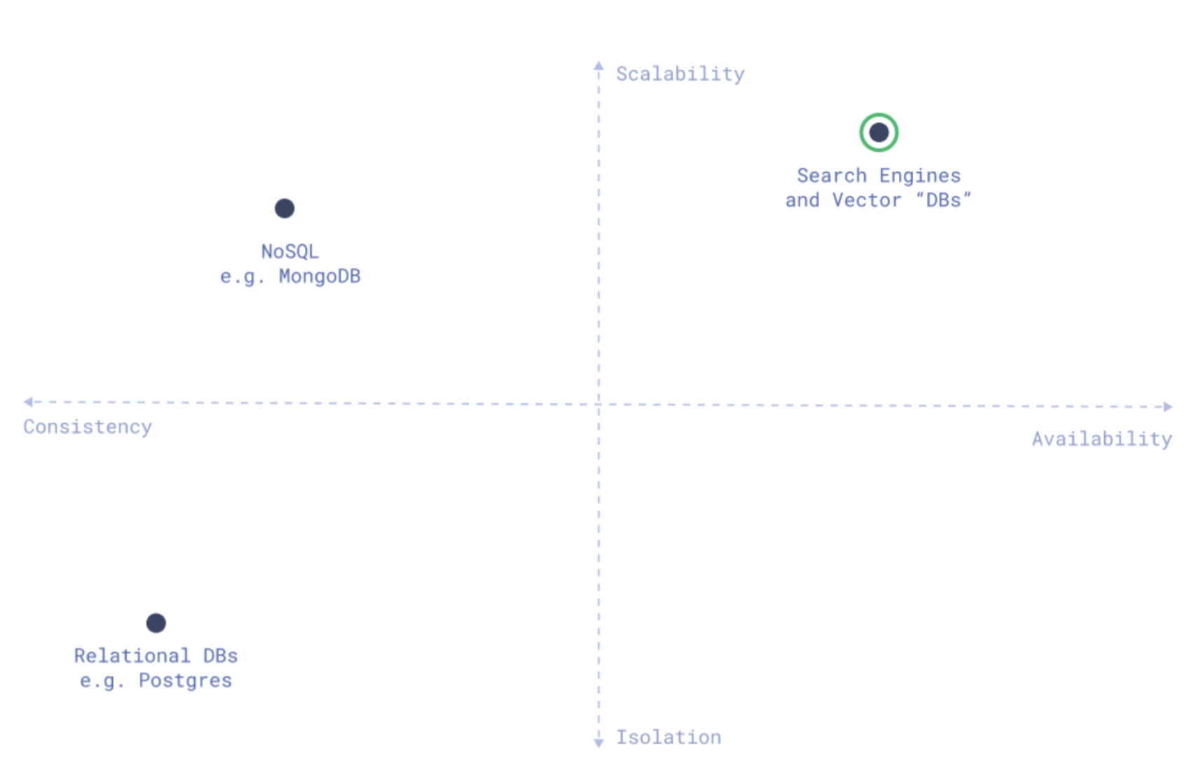
A mapping of database types among main database properties: Source
Based on the data type and prioritization, different database types are suitable for specific scenarios:
Vector Database
Vector Search Extension / Integration
Proprietary
Open-Source
A table of available providers of vector databases and vector search add-ons (non-exhaustive, as of 07/25/2024). Source: Author
Using a vector search extension or integration to an existing traditional database (SQL or NoSQL) is generally an easier and quicker transition process because it leverages current database infrastructure and expertise. However, this approach may work best for simple vector search functionality.
As previously mentioned, traditional databases and vector databases are architectured based on different priorities. For instance, relational databases value consistency and isolation of transactions. Whereas vector databases value scalability, search speed, and availability. Having a dedicated vector database also means its operation and maintenance are separate from the existing database, allowing for modularity. Some vector databases may also offer robust monitoring and access control.
Retrofitting vector search capability into traditional databases may compromise performance. Although some traditional database providers are improving their vector search offerings. It depends on your vector dataset (size, dimensions, etc.) and the provider. There are benchmarking tools and libraries available, such as open-source VectorDBBench. Some common vector search performance metrics are:
The following are some benchmarking results from Zilliz, which offers a vector database solution, and Redis, which offers vector search integration.
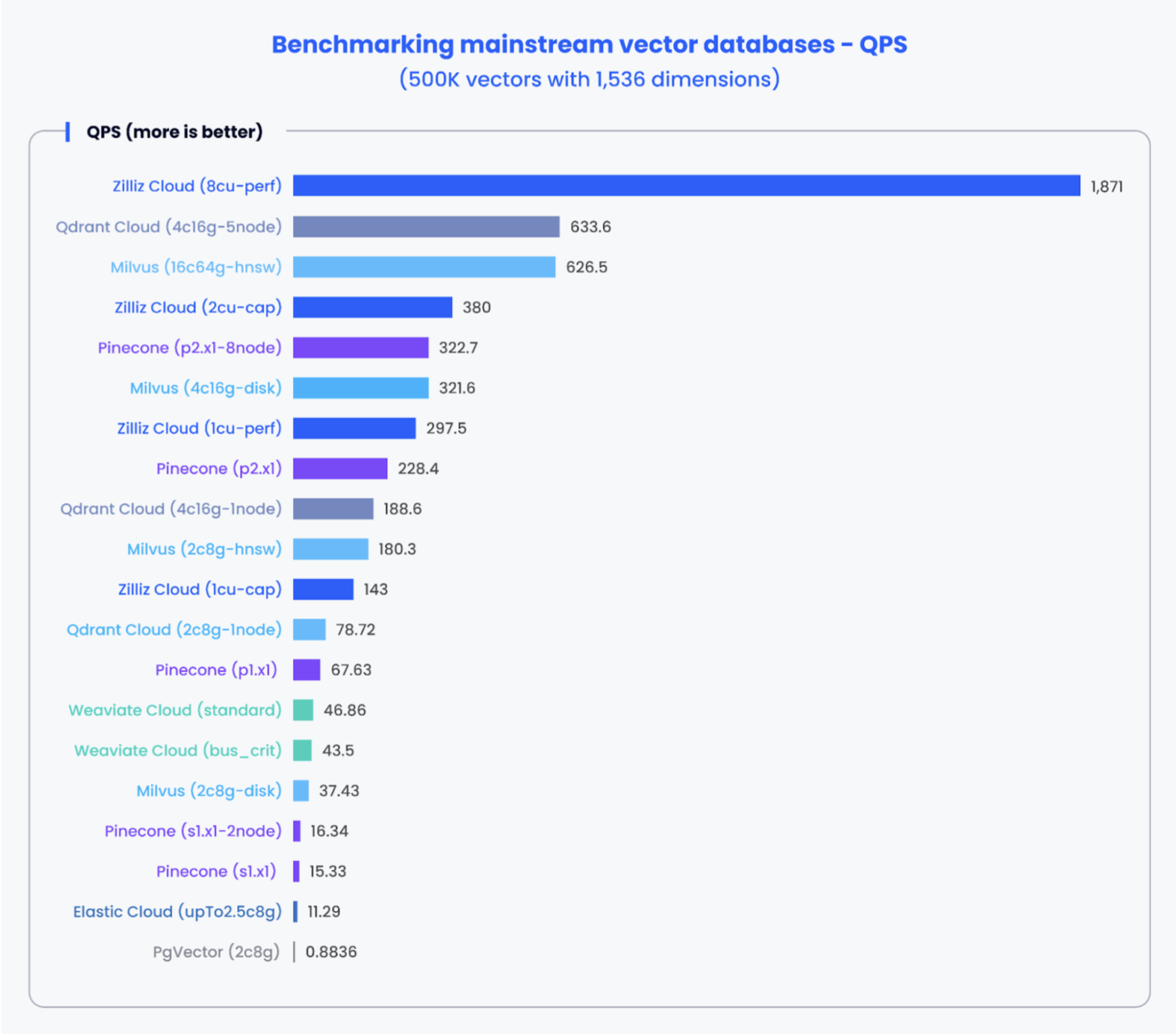
A graph of benchmarking mainstream vector databases and pgvector based on queries per second by Zilliz: Source
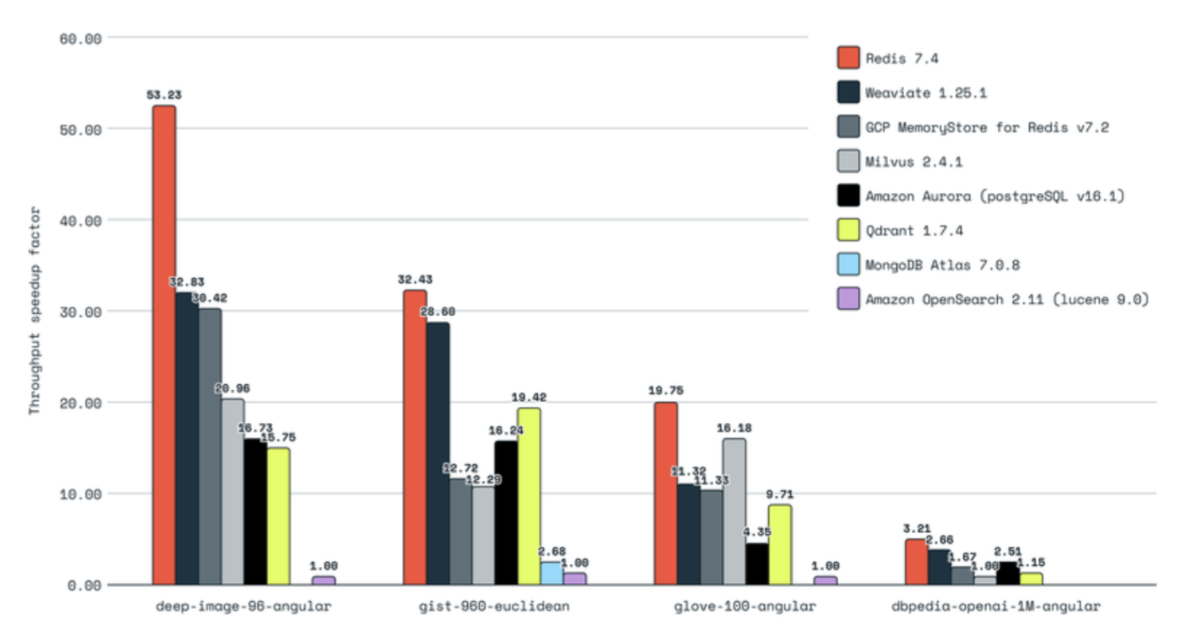
A graph of benchmarking mainstream vector databases and Redis based on throughput speed by Redis: Source
Ultimately, the decision to use a vector database vs. a vector search add-on depends on your application's specific needs for embeddings storage and retrieval. For a small number of embeddings requiring simple vector search capability or to build a prototype, perhaps begin with an extension or integration. As your production system scales, consider setting up a separate vector database for performance optimization and flexibility.
Due to their purpose and architecture, vector databases face the following challenges:
Vector databases, crucial for implementing RAG to enhance an LLM's knowledge, store and retrieve high-dimensional embeddings. They use specialized indexing algorithms for efficient ANN searches, such as IVF, LSH, ANNOY, HNSW, RP, PQ, and SQ. Unlike traditional databases that look for exact matches, vector databases search for similar matches using measures like Euclidean distance, Manhattan distance, cosine similarity, or dot product. Compared to SQL and NoSQL databases, vector databases prioritize scalability and availability, thus optimized for handling unstructured data in AI/ML applications. While vector search add-ons offer a quicker transition, dedicated vector databases may provide better performance and flexibility. Common challenges for vector databases include scaling, fresh data, and containing costs. This is an evolving space with rapid changes, so stay updated.

Explore CS Prep further in our beginner-friendly program.
Get more free resources and access to coding events every 2 weeks.

Connect with one of our graduates/recruiters.

Our graduates/recruiters work at:

Diana Cheung (ex-LinkedIn software engineer, USC MBA, and Codesmith alum) is a technical writer on technology and business. She is an avid learner and has a soft spot for tea and meows.

Connect with one of our recruiters to learn about their journeys.
Our graduates/recruiters work at: